P-values, False Discovery Rate (FDR) and q-values

What are p-values?

The object of differential 2D expression analysis is to find those spots which show expression difference between groups, thereby signifying that they may be involved in some biological process of interest to the researcher.

Due to chance, there will always be some difference in expression between groups. However, it is the size of this difference in comparison to the variance (i.e. the range over which expression values fall) that will tell us if this expression difference is significant or not.

Thus, if the difference is large but the variance is also large, then the difference may not be significant. On the other hand, a small difference coupled with a very small variance could be significant. We use the one way ANOVA test (equivalent t-test for two groups) to formalise this calculation. The tests return a p-value that takes into account the mean difference and the variance and also the sample size.

The p-value is a measure of how likely you are to get this spot data if no real difference existed. Therefore, a small p-value indicates that there is a small chance of getting this data if no real difference existed and therefore you decide that the difference in group expression data is significant. By small we usually mean 0.05.

What are q-values, and why are they important?

False positives

A positive is a significant result, i.e. the p-value is less than your cut off value, normally 0.05.

A false positive is when you get a significant difference when, in reality, none exists. As mentioned above, the p-value is the chance that this data could occur given no difference actually exists. So, choosing a cut off of 0.05 means there is a five per cent chance that the wrong decision is made.

The multiple testing problem

When we set a p-value threshold of, for example, 0.05, we are saying that there is a five per cent chance that the result is a false positive.

In other words, although we have found a statistically significant result, in reality, there is no difference in the group means. While five per cent is acceptable for one test, if lots of tests are performed on the data, then this five per cent can result in a large number of false positives.

For example, if there are 200 spots on a gel and we apply an ANOVA or t-test to each, then we would expect to get 10 false positives by chance alone. This is known as the multiple testing problem.

Multiple testing and the false discovery rate (FDR)

While there are a number of approaches to overcoming the problems due to multiple testing, they all attempt to assign an adjusted p-value to each test, or similarly, reduce the p-value threshold.

Many traditional techniques such as the Bonferroni correction are too conservative in the sense that while they reduce the number of false positives, they also reduce the number of true discoveries.

The False Discovery Rate approach is a more recent development. This approach also determines adjusted p-values for each test. However, it controls the number of false discoveries in those tests that result in a discovery (i.e. a significant result). Because of this, it is less conservative that the Bonferroni approach and has greater ability (i.e. power) to find truly significant results.

Another way to look at the difference is that a p-value of 0.05 implies that five per cent of all tests will result in false positives. An FDR adjusted p-value (or q-value) of 0.05 implies that five per cent of significant tests will result in false positives. The latter is clearly a far smaller quantity.

What are q-values?

q-values are the name given to the adjusted p-values found using an optimised FDR approach.

The FDR approach is optimised by using characteristics of the p-value distribution to produce a list of q-values. In what follows we tie up some ideas and hopefully this will help clarify some of the ideas about p- and q- values.

It is usual to test many hundreds or even thousands of spot variables in a proteomics experiment. Each of these tests will produce a p-value.

The p-values take on a value between 0 and 1 and a histogram can be created to get an idea of how the p-values are distributed between 0 and 1.

Some typical p-value distributions are shown in the images below.

On the x-axis we have histogram bars representing p-values. Each has a width of 0.05 and so in the first bar (red or green) those p-values are between 0 and 0.05.

Similarly, the last bar represents those p-values between 0.95 and 1.0, and so on. The height of each bar gives an indication of how many values are in the bar. This is called a density distribution because the area of all the bars always adds up to 1.

Although the two distributions appear quite different, you’ll notice that they flatten off towards the right of the histogram. The red (or green) bar represents the significant values, if you set a p-value threshold of 0.05.

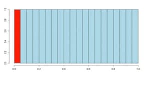
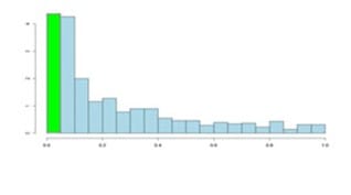
If there are no significant changes in the experiment, you will expect to see a distribution more like the chart with a red bar on the image above. While an experiment with significant changes will look more like the second image witth the green bar.

So, even if there are no significant changes in the experiment, we still expect, by chance, to get p-values < 0.05. These are false positives, and shown in red.

Even in an experiment with significant changes (in green), we are still unsure if a p-value < 0.05 represents a true discovery or a false positive.

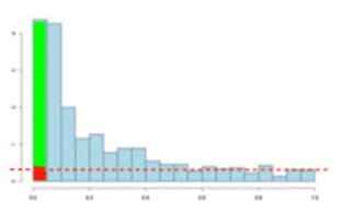
Now, the q-value approach tries to find the height where the p-value distribution flattens out and incorporates this height value into the calculation of FDR adjusted p-values.

This can be seen in the histogram below. This approach helps to establish just how many of the significant values are actually false positives (the red portion of the green bar).

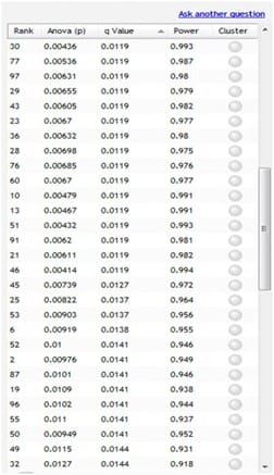
Now, the q-values are simply a set of values that will lie between 0 and 1. Also, if you order the p-values used to calculate the q-values, then the q-values will also be ordered. This can be seen in the following screen shot from SameSpots. Notice that q-values can be repeated.

Interpreting q-values

To interpret the q-values, you need to look at the ordered list of q-values. There are 839 spots in this example experiment.

If we take spot 52 as an example, we see that it has a p-value of 0.01 and a q-value of 0.0141. Recall that a p-value of 0.01 implies a one per cent chance of false positives, and so with 839 spots, we expect between 8 or 9 false positives, on average, i.e. 839*0.01 = 8.39.

In this experiment, there are 52 spots with a value of 0.01 or less, and so 8 or 9 of these will be false positives. On the other hand, the q-value is a little greater at 0.0141, which means we should expect 1.41 per cent of all the spots with q-value less than this to be false positives. This is a much better scenario.

We know that 52 spots have a q-value less than 0.0141 and so we should expect 52*0.0141 = 0.7332 false positives, i.e. less than one false positive.

Just to reiterate, false positives according to p-values take all 839 values into account when determining how many false positives we should expect to see, while q-values take into account only those tests with q-values less the threshold we choose.

Of course, it is not always the case that q-values will result in less false positives, but what we can say is that they give a far more accurate indication of the level of false positives for a given cut-off value.

When doing lots of tests, as in a proteomics experiment, it is more intuitive to interpret p and q values by looking at the entire list of values in this way rather than looking at each one independently.

In this way, a threshold of 0.05 has meaning across the entire experiment. When deciding on a cut-off or threshold value, you should do this from the point of view of how many false positives will this result in, rather than just randomly picking a p- or q-value of 0.05 and saying that everything with a value less than this is significant.