
Western blot densitometry: how band quantification works

Western blot densitometry is the measurement of a band’s integrated pixel intensity after background subtraction, expressed relative to a loading control or to total lane protein. It is how a blot image becomes a number. Most methods sections cover it in one clause, some version of “band intensities were quantified by densitometry”, and that clause hides every decision that changes the result. This guide takes those decisions in order. It covers what band intensity actually measures, why saturation and the linear range decide whether the number means anything, how much background subtraction moves the result, the calculation from raw image to ratio to control, and how to report it so a reviewer can reproduce it. The worked example uses the same arithmetic in ImageJ, in an imager’s bundled software or in Phoretix 1D.
Densitometry is one part of the job. For the whole workflow, from planning the load to reporting fold change across replicates, see how to quantify a western blot, step by step.

What does western blot densitometry measure? Band intensity, volume and integrated density
Densitometry started as a measurement of optical density on film, which is where the name comes from. On a digital image the software measures pixel intensity instead, but the term stayed. Three terms for the measured quantity appear in papers and software, alongside two things people confuse with it.
Band intensity, band volume and integrated density all describe the same thing: the sum of pixel intensities inside the band’s boundary, after the background contribution has been removed. “Volume” is the word most gel software uses, because the software treats the band as a three-dimensional peak and measures the volume under it. “Integrated density” is ImageJ’s name for it. Papers most often write “band intensity.” Whichever word you use, report the integrated value, not the peak height or the mean pixel value, because integrated intensity is the only one of the three that scales with the amount of protein across a range of band shapes.
The lane profile is the one-dimensional trace you get by summing pixel intensity across the width of a lane at every position down its length. Each band appears as a peak. Densitometry on a lane profile means measuring the area under each peak above a baseline. Lane-based software builds this profile automatically; in ImageJ you draw the rectangle and plot it.
The image itself matters more than the software. Quantify the raw acquisition file from your imager, saved as an uncompressed 16-bit TIFF where the instrument offers it, never a JPEG or a screenshot. JPEG compression alters pixel values, and 8-bit images have 256 intensity levels against 65,536 in 16-bit, which limits the dynamic range you can quantify over. Some free tools analyze 8-bit images only; GelAnalyzer vs Phoretix 1D shows what that does to a faint band. Phoretix 1D reads 8-bit and 16-bit uncompressed TIFF from any imager, so the analysis starts from the raw data rather than a compressed export.
Saturation and the linear range: check these before you quantify anything
A densitometry value is only meaningful if the signal was captured in the range where intensity is proportional to protein amount. Two things break that proportionality, and both have to be checked before the calculation, not after.
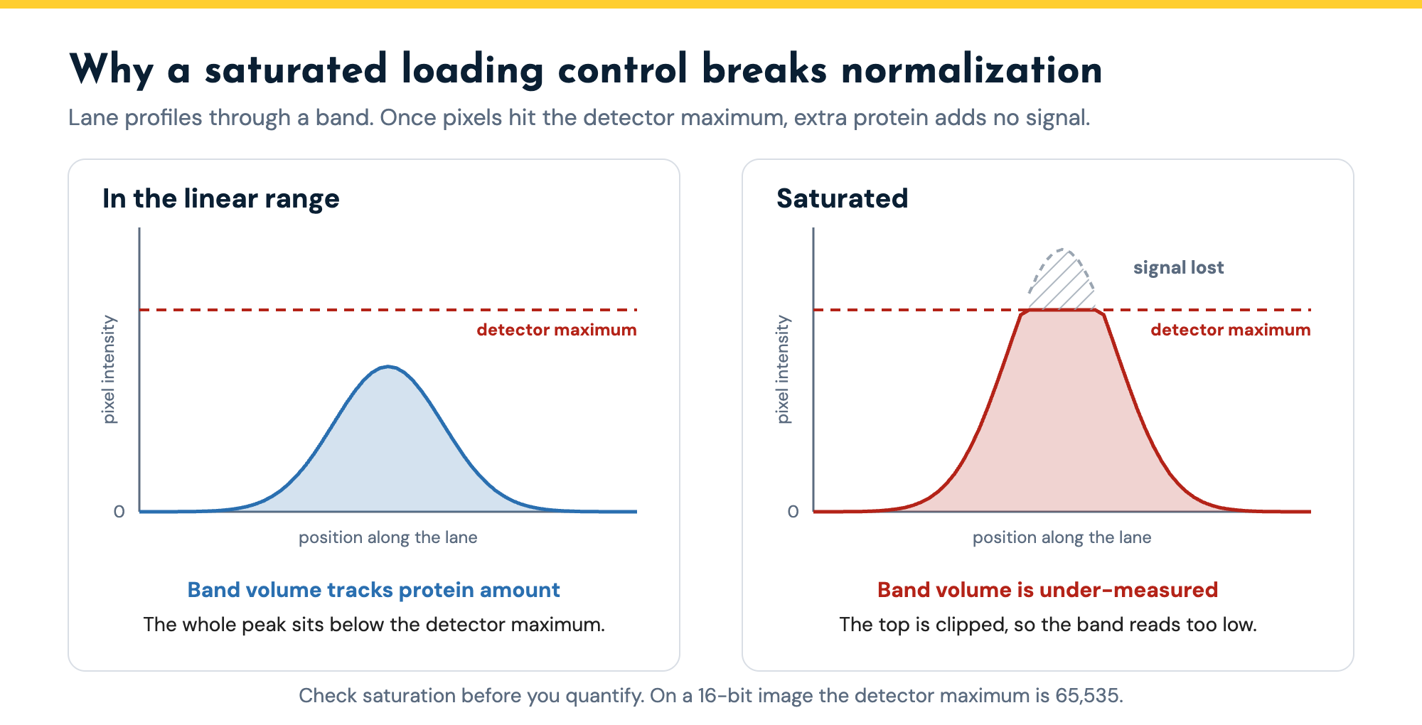
Saturation is the first. Every detector has a maximum value it can record; on a 16-bit camera that is 65,535. Once a band’s brightest pixels hit that ceiling, more protein produces no more signal, and the band’s measured intensity is capped. A saturated band will always be under-quantified, which compresses the difference between your strongest samples and everything else. Chemiluminescent (ECL) detection saturates readily, because the signal is bright and the exposure is often set to make faint bands visible. Fluorescent detection generally has a wider linear range, which is one reason quantitative labs move to it, but it saturates too. Most imagers can display saturated pixels as a colored overlay; check it on every blot and re-expose for a shorter time if any band you intend to quantify is flagged. On film the problem is worse and less visible: film has a narrow linear response and saturates as a smooth roll-off rather than a hard ceiling, which is one reason journals now expect digital acquisition for quantitative work.
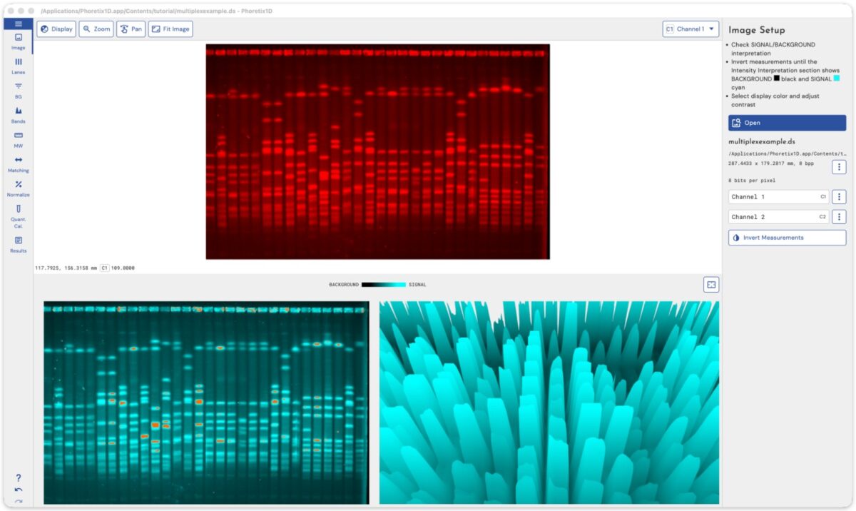
Phoretix 1D shows the same check on the image itself. Its 3D view plots every pixel’s intensity as height, so a saturated band stands out as a flat-topped peak before you quantify anything.
The linear range is the second. Even below saturation, signal is proportional to protein only over a limited loading range, and that range differs between antibodies, substrates and detection methods. The standard way to establish it is a dilution series of one sample, typically five to eight two-fold dilutions, blotted and detected exactly as your experiment will be. Plot band intensity against amount loaded; the linear portion is your working range, and every sample you quantify should fall inside it. Journals including the Journal of Biological Chemistry ask authors to demonstrate this for quantitative blots. Loading controls need the same check: abundant housekeeping proteins such as beta-actin and GAPDH saturate at loadings where the target is still faint, which is the most common way a normalization goes wrong.
If a band is already saturated, or the blot has other problems such as high background or smeared bands, the western blot troubleshooting guide shows which problems you can still quantify and which need a re-image or a re-run.
Western blot densitometry calculation, step by step
The calculation is the same in any software. What differs is how much of it is automated and how much depends on where an operator draws a box.
- Acquire the image in the linear range. Use the raw 16-bit file, confirm no quantified band is saturated, and keep the exposure identical for every blot you intend to compare.
- Define the lanes. Automated lane detection finds each lane’s boundaries from the image; in ImageJ you draw an identical rectangle around each lane by hand. Lanes on a warped or “smiling” gel need boundaries that follow the distortion, which manual rectangles cannot do.
- Detect the bands. Each band becomes a peak in the lane profile with a start and end position. Automated detection applies the same sensitivity to every lane; manual detection asks the operator to judge where each band begins and ends.
- Subtract the background. Choose one method (see the next section) and apply it identically to every lane and every blot in the comparison. This single choice changes the final number more than any other.
- Measure band intensity. Record the integrated intensity (volume) of each target band and each loading-control band after background subtraction.
- Normalize. Divide each target band by its loading control from the same lane, either the housekeeping band (beta-actin, GAPDH, tubulin) or the total protein in that lane from a total-protein stain. This corrects for differences in the amount loaded.
- Express the result relative to your control. Divide each normalized value by the normalized value of the control condition. The control becomes 1.0 and every other sample is a ratio to control, which is the same thing as fold change.
- Repeat across biological replicates and apply your statistics to the ratios, not to the raw intensities.
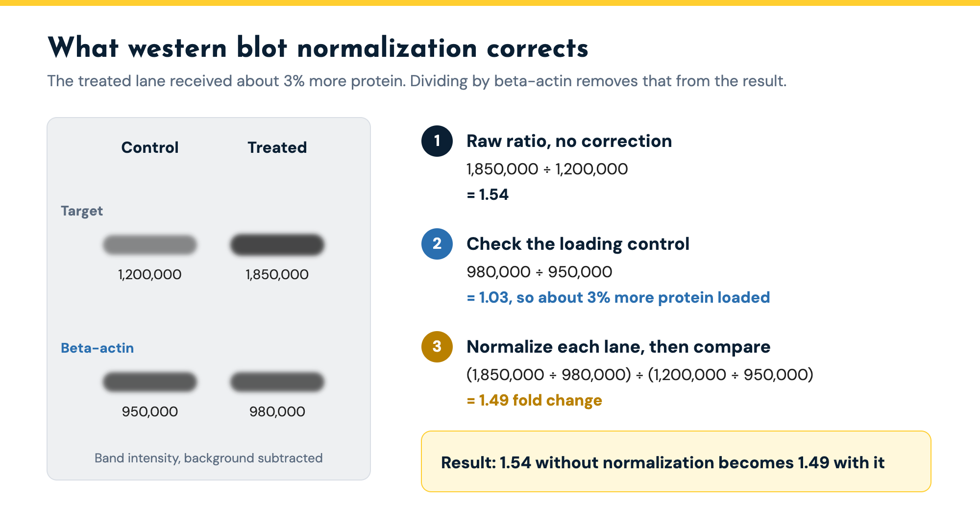
The table below runs the arithmetic on two lanes. Look at the beta-actin row. The treated lane received about 3% more protein than the control lane, and without normalization that alone would push the ratio from 1.49 to 1.54.
| Step | Control lane | Treated lane | Note |
|---|---|---|---|
| Target band volume (background subtracted) | 1,200,000 | 1,850,000 | Integrated intensity inside the band boundary after background subtraction; arbitrary units |
| Beta-actin band volume (background subtracted) | 950,000 | 980,000 | Same lane as the target; same background method; confirmed in the linear range by a dilution series |
| Normalized intensity (target divided by beta-actin) | 1.263 | 1.888 | Corrects for the amount of protein that actually reached each lane |
| Ratio to control (normalized value divided by the control's normalized value) | 1.00 | 1.49 | The control becomes 1.0; the treated sample shows a 1.49-fold increase |
| For comparison: raw ratio with no normalization | 1.00 | 1.54 | The treated lane received about 3% more protein, which inflates the unnormalized ratio |
A worked western blot densitometry calculation for one target protein in a control and a treated lane, normalized to beta-actin and expressed as a ratio to control. Intensities are integrated band volumes in arbitrary units after background subtraction.
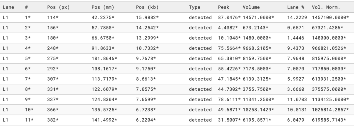
Phoretix 1D produces these numbers for you. Its results table lists the background-subtracted volume and normalized volume of every band in every lane, ready to export to CSV.
Background subtraction: the choice that changes your number
No membrane is perfectly blank. Substrate glow, non-specific antibody binding, film fog and uneven transfer all add intensity that has nothing to do with your protein, and it is rarely uniform across the blot. Background subtraction estimates that contribution under each band and removes it. The estimate depends on the method, and for some methods on where the operator clicks, which makes it the largest source of person-to-person variation in densitometry. The table below compares the methods.
| Method | How it estimates the background | Works well for | Watch out for |
|---|---|---|---|
| None | No subtraction; the full integrated intensity inside the band boundary is reported | Images already background-corrected at acquisition, or a deliberate check of what subtraction is removing | Membrane background, substrate glow and film fog inflate every band, and unevenly, so ratios between lanes are unreliable |
| Rolling ball | A virtual ball of a set radius is rolled beneath the lane's intensity profile; the surface it traces is treated as background and subtracted | Most blots and gels, especially those with a background that varies gradually across the membrane; no reference region needs to be chosen | The ball radius must be larger than the width of your widest band, or the method removes real signal as if it were background; use one radius for the whole comparison |
| Profile minimum | The lowest intensity value found in the lane profile is taken as the background level and subtracted along the whole lane | Clean images with a flat, even background where the lane's emptiest point is a fair estimate of background everywhere | One dark artifact or dust speck sets the baseline too low and inflates every band; a background gradient along the lane is not followed |
| Constant value | A fixed value chosen by the operator, typically measured from a blank region of the image, is subtracted from every pixel | Uniform backgrounds where a single value represents the whole membrane, and validated protocols where the value is fixed and documented | The same value applied to lanes with different local background over- or under-corrects them; record the value and how it was chosen |
| Rubber band | A line is stretched beneath the lane profile so that it touches the lowest points between peaks, like an elastic band under the trace, and everything below it is subtracted | Profiles with distinct, well-separated peaks and a baseline that drifts along the lane; no radius or value to set | Broad or closely spaced peaks lift the band so it cuts into real signal; doublets and smears are the usual failure |
| Image rectangle | The operator draws a rectangle over an empty region of the image, such as an unused lane; the average pixel intensity inside it is subtracted as a constant background | Images with a clearly empty reference region and an even background, when you want one documented background value measured from the image itself | The rectangle must sit on truly empty membrane; a smear, an edge artifact or a region too close to a lane sets the wrong value for every band, and a gradient across the blot is not followed |
| Lane edge | At each point down the lane, the lower of the two pixel values at the edges of the lane is taken as the background and subtracted | Western blots and DNA gels with multiple tightly spaced bands; when the lane is wider than the bands, it is very effective at removing co-migrating material | Bands must sit completely inside the lane boundary; if a lane edge cuts through a band, that band material is subtracted as background and the band is severely under-measured |
| Manual | The operator defines the background under each band by hand | Rescuing individual lanes where an artifact defeats every automated method | The largest source of operator-to-operator variation in densitometry; document every manual adjustment and avoid it for routine quantification |
The background subtraction methods available in Phoretix 1D, how each estimates the background under a band, where it works well and what to watch for. ImageJ offers rolling ball and a hand-drawn baseline.
Two rules hold regardless of method. Apply the same method with the same settings to every lane in a comparison, because switching methods between lanes changes the result more than the biology does. And write the method into your methods section, because “background subtracted” on its own is not reproducible. Rolling ball is a common default for blots because it follows a gradually varying background without the operator choosing a reference region. Its one parameter, the ball radius, must be larger than the width of your bands, or it subtracts real signal as if it were background. Phoretix 1D offers six background methods (none, rolling ball, profile minimum, a constant user-defined value, rubber band and fully manual) and applies the chosen one to every lane at once, so no lane is treated differently from its neighbors.
Normalization: the step after densitometry
Densitometry gives you a band intensity. Normalization turns it into a comparison, by dividing the target by a loading control from the same lane to correct for the protein that actually reached each lane. There are two kinds of loading control. A housekeeping band (beta-actin, GAPDH or tubulin) is what most published methods still describe; in our analysis of papers citing TotalLab software, beta-actin is named in about one in six. Total protein in the lane, from a stain-free gel or a membrane stain such as Ponceau S or REVERT, is less sensitive to any one protein changing with your treatment and has a wider linear range, and reagent manufacturers now recommend it for quantitative blots. The total protein normalization guide compares stain-free, Ponceau S and fluorescent stains and shows how to capture a valid total protein image.
Whichever you use, three rules carry over from densitometry. The loading control comes from the same lane. It has to be in its own linear range, which abundant housekeeping proteins often are not at normal loadings. And it is quantified with the same background method as the target. The normalization guide covers both methods, a worked total-protein calculation, the case where the two disagree, and a calculator.
Densitometry in ImageJ versus dedicated software
ImageJ and Fiji can do every step above, and they are free, which is why ImageJ was named in about one in five of the recent western blot papers we sampled. The gel analysis tool in ImageJ works from rectangles you draw around each lane, plots the lane profile, and lets you draw a baseline under each peak with the line tool before measuring the area with the wand. Every one of those actions is a judgment: the rectangle position, the rectangle size, where the baseline goes. Two people quantifying the same blot in ImageJ will usually get different numbers, and the same person can get different numbers on different days. The results then go to a spreadsheet for background, normalization and ratio calculations by hand.
Dedicated 1D analysis software automates the judgments. Lanes and bands are detected by algorithm and applied identically across the blot; background subtraction is a named method with a recorded parameter; normalization and ratio to control are built in and exported; and the whole analysis is saved with the image so it can be reopened, audited or rerun. The gain is reproducibility. Any operator, on any day, gets the same number from the same image. For regulated labs, Phoretix 1D with TotalLab’s AuditSafe module adds audit trails, electronic signatures, user permissions and image authenticity checks for FDA 21 CFR Part 11 and EU Annex 11, which ImageJ has no equivalent for.
Phoretix 1D is TotalLab’s dedicated software for this work. It runs on Windows, macOS and Linux, opens raw files from any imager, and produces the densitometry, normalization and ratio-to-control results above in one pass with a PDF report and CSV export. The software comparison guide sets it beside ImageJ, Image Lab, Empiria Studio, iBright and GelAnalyzer.
How to report densitometry in your methods section
Most methods sections compress densitometry into a single sentence, and most reviewers accept it, but the sentence should carry enough to be reproduced. A complete version names the image source, the software and version, the background method, the normalization, and how the result is expressed:
“Blots were imaged on a [imager] and band intensities were quantified by densitometry using Phoretix 1D version [X] (TotalLab Ltd, Newcastle upon Tyne, UK). Background was subtracted using the rolling ball method. Band intensities were normalized to [beta-actin / total protein in the same lane] and expressed as a ratio to the [control condition]. All samples were confirmed to lie within the linear range of detection by a dilution series.”
State the number of biological replicates and the statistical test applied to the normalized ratios in the figure legend. If any band was excluded for saturation, say so. Many journals now ask for the uncropped blots and the linear-range evidence as supplementary data; keep the raw TIFF files and the saved analysis so you can supply them.
To cite the software: Phoretix 1D (TotalLab Ltd, Newcastle upon Tyne, UK), with the version number you used. TotalLab’s earlier 1D products, TotalLab Quant, TL120 and TL100, are still widely cited from older installations; if your lab has upgraded, cite Phoretix 1D so your methods match the software you ran.
Frequently asked questions
Q: What is densitometry in a western blot?
A: Densitometry is the measurement of how much signal each band contains, taken from the blot image as the sum of pixel intensities inside the band after background has been subtracted. That integrated intensity, also called band volume or integrated density, is proportional to the amount of protein in the band as long as the signal was captured in the detector’s linear range. It is then normalized to a loading control and expressed as a ratio to the control condition.
Q: How do you calculate western blot densitometry?
A: Measure the background-subtracted integrated intensity of the target band and of the loading-control band in the same lane. Divide target by loading control to get the normalized intensity. Divide each sample’s normalized intensity by the control sample’s normalized intensity; the control becomes 1.0 and each sample is a ratio to control, or fold change. Repeat for each biological replicate and run statistics on the ratios.
Q: What is the difference between band intensity, band volume and integrated density?
A: Nothing in substance. All three mean the sum of pixel intensities within the band boundary after background subtraction, although ImageJ’s integrated density includes the background unless you subtract it first. “Volume” is the usual term in gel analysis software, “integrated density” is ImageJ’s term, and “band intensity” is what most papers write. Avoid reporting peak height or mean pixel value, which do not scale reliably with protein amount.
Q: Does a saturated band matter if I am only comparing lanes?
A: Yes. A saturated band is under-measured because its brightest pixels have hit the detector ceiling, so the difference between it and a weaker band is compressed and the ratio you calculate is wrong. Check the saturation overlay on your imager, re-expose for a shorter time, and never quantify a band that shows saturated pixels.
Q: Is western blot densitometry quantitative or semi-quantitative?
A: Usually semi-quantitative. Densitometry gives the relative amount of a protein between lanes on the same blot, expressed as a ratio to control, not an absolute mass in nanograms. It becomes quantitative in the stricter sense only when a standard curve of purified protein is run on the same blot and every sample falls inside its linear range. Either way, the ratios are only valid if no band is saturated and the same background method is applied to every lane.
Q: Can I do western blot densitometry in ImageJ?
A: Yes. ImageJ’s gel analysis tool plots a lane profile from a hand-drawn rectangle and measures the area under each peak above a hand-drawn baseline. The limitation is reproducibility: the rectangle, the baseline and the background are all operator judgments, so different people get different numbers from the same blot. Dedicated software automates those choices and saves them with the analysis.
Q: What software is used for western blot densitometry?
A: ImageJ and Fiji, the software bundled with imagers (Bio-Rad Image Lab, LI-COR Empiria Studio, Thermo Fisher iBright Analysis Software), free tools such as GelAnalyzer, and independent packages such as TotalLab’s Phoretix 1D, which reads images from any imager and runs on Windows, macOS and Linux. The software comparison guide on this site compares them on lane and band detection, background subtraction, normalization, file formats and compliance.
Q: How do I describe densitometry in a methods section?
A: Name the imager, the software and version, the background subtraction method, the normalization (which loading control or total protein), and how results are expressed (ratio to control or fold change), and state that samples were within the linear range. A template sentence is given in the reporting section above.
Get the same densitometry number from every operator
Phoretix 1D detects lanes and bands automatically, applies one background method across the whole blot, normalizes to a housekeeping band or total protein, and reports ratio to control with a PDF and CSV in one pass. Free trial, any imager, Windows, macOS and Linux.
References
- Gassmann M, Grenacher B, Rohde B, Vogel J. Quantifying Western blots: pitfalls of densitometry. Electrophoresis. 2009;30(11):1845-1855. DOI 10.1002/elps.200800720.
(Source for: saturation, film versus digital response, background subtraction as a source of error, definition of densitometry.) - Taylor SC, Posch A. The design of a quantitative western blot experiment. BioMed Research International. 2014;2014:361590. DOI 10.1155/2014/361590.
(Source for: linear dynamic range and the dilution series, loading-control saturation, total protein normalization.) - Pillai-Kastoori L, Schutz-Geschwender AR, Harford JA. A systematic approach to quantitative Western blot analysis. Analytical Biochemistry. 2020;593:113608. DOI 10.1016/j.ab.2020.113608.
(Source for: establishing the linear range, housekeeping protein limitations, total protein normalization, fluorescent versus chemiluminescent linear range.) - Fosang AJ, Colbran RJ. Transparency is the key to quality. Journal of Biological Chemistry. 2015;290(50):29692-29694. DOI 10.1074/jbc.E115.000002.
(Source for: journal expectations for quantitative western blots, linear range evidence and uncropped blots.) - Schneider CA, Rasband WS, Eliceiri KW. NIH Image to ImageJ: 25 years of image analysis. Nature Methods. 2012;9:671-675. DOI 10.1038/nmeth.2089.
(Source for: ImageJ.) - Sternberg SR. Biomedical image processing. Computer. 1983;16(1):22-34. DOI 10.1109/MC.1983.1654163.
(Source for: the rolling ball background algorithm.) - TotalLab. Phoretix 1D product page. https://totallab.com/software/1d-gel-western-blot-analysis-software/
(Source for: 8-bit and 16-bit TIFF; images from any imager; Windows, macOS and Linux; PDF report and CSV export; normalization modes.) - TotalLab product team, September 2026 (internal).
(Source for: Phoretix 1D background subtraction options: none, rolling ball, profile minimum, constant (user-defined value), rubber band and fully manual.) - TotalLab customer-language analysis of 2,907 papers citing TotalLab 1D software, 2001 to 2026, and full text of 487 open-access papers, September 2026 (internal).
(Source for: “densitometry” as the most common analysis term; beta-actin named in about one in six citing contexts; TotalLab Quant, TL120 and TL100 still cited from older installations.) - TotalLab Language Audit, 15 September 2026 (internal): 66 recent western blot papers from PubMed, with full text where open access.
(Source for: ImageJ named in about one in five, 21%, of sampled western blot papers.) - TotalLab. AuditSafe compliance wording, as used on totallab.com.
(Source for: audit trails, electronic signatures, user permissions and image authenticity verification for FDA 21 CFR Part 11 and EU Annex 11.)